
本文主要从以下几个方面介绍如何将时间序列的预测转化为有监督的机器学习问题:
- 数据预处理(数据转换、缺失值、异常值)
- 特征提取(窗口特征、日期特征、时间偏移特征)
- 模型检验(时间序列的交叉验证)
数据预处理
第一步先对时间序列进行观察,看其是否存在缺失值,并结合实际情况对缺失值进行处理或填充。使用的数据下载可点击此处,提取码为fgwa
import pandas as pd
import numpy as np
import matplotlib.pyplot as plt
prices = pd.read_csv("data.txt",sep='\s+')
prices['date']=pd.to_datetime(prices['date'])
prices = prices.set_index('date')
prices.plot(legend=True)  #左图
plt.tight_layout()
plt.show()
### 对缺失值进行时间插值
def interpolate_and_plot(prices, interpolation):
    # Interpolate the missing values
    prices_interp = prices.interpolate(interpolation)
    # Plot the results
    fig, ax = plt.subplots(figsize=(10, 5))
    prices_interp.plot(alpha=.6, ax=ax, legend=True)
    # Now highlight the interpolated values in red
    missing_values = prices.isna() # Create a boolean mask for missing values
    prices_interp[missing_values].plot(ax=ax, color='r', lw=2, legend=False)
    plt.show()
    return prices_interp
# Interpolate linearly
interpolation_type = "linear"
prices = interpolate_and_plot(prices, interpolation_type)  #右图
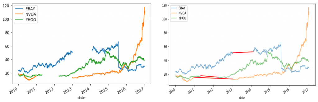
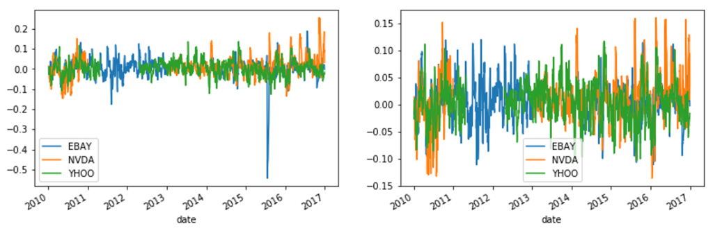
可以看出这三个序列都具有比较明显的不平稳特征,可以进行一定的转换减弱序列的不稳定性。因为数据是股票价格数据,这里使用Pandas中的rolling函数将当前价格转换为当前价格较前一段时间平均价格的增长率。经过转换后也可以更容易地看出异常点所在。
def percent_change(series):
    # Collect all but the last value of this window, then the last value
    previous_values = series[:-1]
    last_value = series[-1]
    # Calculate the % difference between the last value and the mean of earlier values
    percent_change = (last_value - np.mean(previous_values)) / np.mean(previous_values)
    return percent_change
### Apply rolling window and plot
prices_perc = prices.rolling('20d', closed='both').apply(percent_change)
prices_perc.plot()  #下方左图
plt.show()
若数据落在距离均值的三个标准差之外,则判断为异常点。异常点的判断方法有很多,这里仅选用这一简单的准则用做说明。
def replace_outliers(series):
    # Calculate the absolute difference of each timepoint from the series mean
    absolute_differences_from_mean = np.abs(series - np.mean(series))
    # Calculate a mask for the differences that are > 3 standard deviations from zero
    this_mask = absolute_differences_from_mean > (np.std(series) * 3)
    # Replace these values with the median accross the data
    series[this_mask] = np.nanmedian(series)
    return series
# Apply the function to the timeseries and plot the results
prices_perc = prices_perc.apply(replace_outliers)
prices_perc.plot()  #下方右图
plt.show()
特征提取
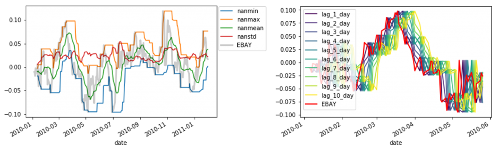
使用Pandas中的rolling函数进行窗口特征的提取,需要注意的是计算窗口特征时不能包含窗口最右边的点,否则提取的特征中就会包含了预测值本身的信息。因此需要将窗口设置为左闭右开的区间 (即参数closed="left")。以EBAY这一列为例:
# Define a rolling window with Pandas, excluding the right-most datapoint of the window
prices_perc_rolling = prices_perc['EBAY'].rolling("20d", min_periods=5, closed='left')
# Define the features that calculate for each window
features_to_calculate = [np.nanmin, np.nanmax, np.nanmean, np.nanstd]
# Calculate these features for rolling window object
features = prices_perc_rolling.aggregate(features_to_calculate)
# Plot the result
ax = features.loc[:"2011-01"].plot()
prices_perc['EBAY'].loc[:"2011-01"].plot(ax=ax, color='k', alpha=.2, lw=3)  #下方左图
ax.legend(loc=(1.01, .6))
plt.show()
如果窗口特征的计算中需要传入参数,可使用partial函数
# Import partial from functools
from functools import partial
percentiles = [1, 10, 25, 50, 75, 90, 99]
# Use a list comprehension to create a partial function for each quantile
percentile_functions = [partial(np.nanpercentile, q=percentile) for percentile in percentiles]
# Calculate each of these quantiles on the data using a rolling window
prices_perc_rolling = prices_perc['EBAY'].rolling("20d", min_periods=5, closed='left')
features_percentiles = prices_perc_rolling.aggregate(percentile_functions)
除去窗口特征外,还可以直接对日期信息进行处理获得新的特征,例如:
prices_perc['day_of_week'] = prices_perc.index.dayofweek
prices_perc['week_of_year'] = prices_perc.index.weekofyear
prices_perc['month_of_year'] = prices_perc.index.month
除去窗口特征和日期特征外,还可以直接使用离预测时刻最近的过去几个时刻的值作为特征,使用Pandas中的shift函数构建时间偏移特征。
# These are the "time lags"
shifts = np.arange(1, 11).astype(int)
# Use a dictionary comprehension to create name: value pairs, one pair per shift
shifted_data = {"lag_{}_day".format(day_shift): prices_perc['EBAY'].shift(day_shift) for day_shift in shifts}
# Convert into a DataFrame for subsequent use
prices_perc_shifted = pd.DataFrame(shifted_data)
# Plot the first 100 samples of each
ax = prices_perc_shifted.iloc[:100].plot(cmap=plt.cm.viridis)  #下方右图
prices_perc['EBAY'].iloc[:100].plot(color='r', lw=2)
ax.legend(loc='best')
plt.show()
# Replace missing values with the median for each column
X = prices_perc_shifted.fillna(np.nanmedian(prices_perc_shifted))
y = prices_perc.fillna(np.nanmedian(prices_perc))['EBAY']
模型检验
使用sklearn中的TimeSeriesSplit进行模型的交叉检验,不同于一般的交叉检验,时间序列的交叉检验中验证集始终在训练集之后,如下图所示:
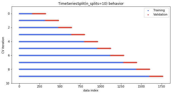
由于时间序列的交叉验证的特殊性,可以将所有交叉验证的结果看作一个时间序列:
from sklearn.model_selection import TimeSeriesSplit
cv = TimeSeriesSplit(n_splits=100)  #Initialize the cross-validation iterator
scores_time = []
for ii, (tr, tt) in enumerate(cv.split(X, y)):
    start_val = tt[0]
    scores_time.append(X.index[start_val])  #the start datetime for each validation set
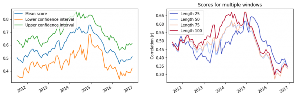
在交叉验证时可以使用自定义的指标来衡量模型的好坏,同时可以使用bootstrap方法来衡量模型的不确定性:
from sklearn.utils import resample
def bootstrap_interval(data, percentile, n_boots=100):
    """Bootstrap a confidence interval for the mean of a 1-D dataset."""
    # Create empty array to fill the results
    bootstrap_means = np.zeros(n_boots)
    for ii in range(n_boots):
        # Generate random indices for data with replacement, then take the sample mean
        random_sample = resample(data)
        bootstrap_means[ii] = random_sample.mean()
    # Compute the percentiles of choice for the bootstrapped means
    data_percentile = np.percentile(bootstrap_means, percentile)
    return data_percentile
def my_pearsonr(est, X, y):
    """Use pearson correlation for validation score"""
    y_pred = est.predict(X).squeeze()
    # Use the numpy "corrcoef" function to calculate a correlation matrix
    my_corrcoef_matrix = np.corrcoef(y_pred, y.squeeze())
    # Return a single correlation value from the matrix
    my_corrcoef = my_corrcoef_matrix[1, 0]
    return my_corrcoef
本文仅使用了时间偏移特征以及岭回归构建机器学习模型,为获得更好的效果,可以使用更多的特征以及更复杂的回归算法。
from sklearn.linear_model import Ridge
from sklearn.model_selection import cross_val_score
# Generate scores for each split to see how the model performs over time
model = Ridge()
cv = TimeSeriesSplit(n_splits=100)
scores = cross_val_score(model, X, y, cv=cv, scoring=my_pearsonr)
# Convert to a Pandas Series object
scores_series = pd.Series(scores, name='score', index=scores_time)
# Bootstrap a rolling confidence interval for the mean score
scores_mean = scores_series.rolling(20).mean()
scores_lo = scores_series.rolling(20).aggregate(partial(bootstrap_interval, percentile=2.5))
scores_hi = scores_series.rolling(20).aggregate(partial(bootstrap_interval, percentile=97.5))
# Plot the results
fig, ax = plt.subplots()
scores_mean.plot(ax=ax, label="Mean score")
scores_lo.plot(ax=ax, label="Lower confidence interval")
scores_hi.plot(ax=ax, label="Upper confidence interval")
ax.legend()
plt.show()  #下方左图
在使用函数TimeSeriesSplit时,还可以通过定义参数max_train_size来限制每个验证集之前使用的训练样本个数:
# Pre-initialize window sizes
window_sizes = [25, 50, 75, 100]
# Create an empty DataFrame to collect the scores
all_scores = pd.DataFrame(index=scores_time)
# Generate scores for each split to see how the model performs over time
for window in window_sizes:
    # Create cross-validation object using a limited lookback window
    cv = TimeSeriesSplit(n_splits=100, max_train_size=window)
    # Calculate scores across all CV splits and collect them in a DataFrame
    this_scores = cross_val_score(model, X, y, cv=cv, scoring=my_pearsonr)
    all_scores['Length {}'.format(window)] = this_scores
# Visualize the scores
ax = all_scores.rolling(20).mean().plot(cmap=plt.cm.coolwarm)
ax.set(title='Scores for multiple windows', ylabel='Correlation (r)')
plt.show()  #下方右图
本文介绍了针对时间序列构造机器学习模型的常用方法,更高级和自动化的时间序列特征生成器可以参考tsfresh