
在文章强化学习:Deep Q-Learning中介绍的方法属于基于价值(Value-Based)的方法,即估计最优的q(s,a),再从q(s,a)中导出最优的策略\pi(例如\epsilon-greedy)。但是有没有方法能不经过中间过程,直接对最优策略进行估计呢?这样做又有什么好处呢?该部分要介绍的就是这类方法,即基于策略(Policy-Based)的方法。下面先介绍一下这类方法的好处:
- 能够处理连续的动作空间(continuous action space)。在强化学习:Deep Q-Learning中可以看出Value-Based方法适合离散有限的动作空间,但对于连续的动作空间就不能很好地处理。
- 能够得到最优的随机策略(stochastic policy)。尽管\epsilon-greedy等方式为策略选择加入了一定的随机性,但本质上Value-Based方法得到的最优策略是确定的,即对于同一状态s,对应同一动作a。下面举两个例子说明随机策略相对于确定策略的优势:
- 假设训练智能体玩石头、剪刀、布的游戏,最终的最优策略就是一个完全随机的策略,不存在确定的最优策略,因为任何固定的套路都可能会被对手发现并加以利用。
- 在和环境的交互过程中智能体常常会遇到同一种状态(aliased states),若对遇到的同一种状态都采用固定的动作有可能得不到最优的结果,特别是当智能体处在一个只能部分感知的环境(Partially Observable Environment)中时。如下图所示,假设智能体的目标是吃到香蕉并且不吃到辣椒,但是它只能感知到与它相邻的格点的状况,在两个灰色的格点时智能体感知到的状况是相同的。假设智能体学习到的确定策略如箭头所示,则若智能体位置在黄框范围内时会出现来回地震荡,这显然不是最优的情况。

问题定义
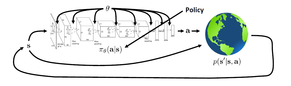
状态和动作集合\tau满足概率函数\tag{1} p_{\theta}(\tau)=p_{\theta}\left(\mathbf{s}_{1}, \mathbf{a}_{1}, \ldots, \mathbf{s}_{T-1}, \mathbf{a}_{T-1}, \mathbf{s}_{T}\right)=p\left(\mathbf{s}_{1}\right) \prod_{t=1}^{T-1}\pi_{\theta}\left(\mathbf{a}_{t} \mid \mathbf{s}_{t}\right) p\left(\mathbf{s}_{t+1} \mid \mathbf{s}_{t}, \mathbf{a}_{t}\right)定义r_{t+1}为状态s_t和动作a_t下获得的奖励,则问题求解可转化为\tag{2} \theta^{\star}=\arg\max_{\theta}J(\theta)=\arg\max_{\theta} \mathbb{E}_{\tau \sim {p_{\theta}(\tau)}}\left[\sum_{t=1}^{T-1} r_{t+1}\right]=\arg\max_{\theta} \mathbb{E}_{\tau \sim {p_{\theta}(\tau)}}r(\tau)容易看出J(\theta)=\int p_{\theta}(\tau) r(\tau) d \tau,采用梯度上升的方法求解J(\theta)的最大值,梯度公式可写为:\tag{3} \begin{aligned}\nabla_{\theta} J(\theta)&=\int \nabla_{\theta} p_{\theta}(\tau) r(\tau) d \tau=\int p_{\theta}(\tau) \nabla_{\theta} \log p_{\theta}(\tau) r(\tau) d \tau=\mathbb{E}_{\tau \sim p_{\theta}(\tau)}\left[\nabla_{\theta} \log p_{\theta}(\tau) r(\tau)\right] \\ &=\mathbb{E}_{\tau \sim p_{\theta}(\tau)} \left[\sum_{t=1}^{T-1} \nabla_{\theta} \log \pi_{\theta}\left(\mathbf{a}_{t} \mid \mathbf{s}_{t}\right)r(\tau)\right] \\ &=\mathbb{E}_{\tau \sim p_{\theta}(\tau)} \left[\sum_{t} \nabla_{\theta} \log \pi_{\theta}\left(\mathbf{a}_{t} \mid \mathbf{s}_{t}\right)\left(\underbrace{\sum_{t^{\prime}=1}^{t-1}r_{t^{\prime}+1}}_{\large b_t}+\underbrace{\sum_{t^{\prime}=t}^{T-1}r_{t^{\prime}+1}}_{\large G_t}\right)\right]\end{aligned}由于b_t与当前动作a_t无关,可令f_{\theta}(s_t)为状态s_t的概率函数,则\tag{4} \begin{aligned} \mathbb{E}_{\tau \sim p_{\theta}(\tau)} \left[\nabla_{\theta} \log \pi_{\theta}\left(\mathbf{a}_{t} \mid \mathbf{s}_{t}\right)b_t\right]&=\int_{s_t} f_{\theta}(s_t)\left[\int_{a_t} \pi_{\theta}\left({a}_{t} \mid {s}_{t}\right) b_t\nabla_{\theta} \log \pi_{\theta}\left({a}_{t} \mid {s}_{t}\right) d a_t\right] d s_t \\ &=\int_{s_t} f_{\theta}(s_t)\underbrace{\left[\nabla_{\theta}\int_{a_t} b_t\pi_{\theta}\left({a}_{t} \mid {s}_{t}\right) d a_t\right]}_{\large b_t\nabla_{\theta}1} d s_t=0 \end{aligned}因此J(\theta)的梯度公式最终可写为\tag{5} \nabla_{\theta} J(\theta)=\mathbb{E}_{\tau \sim p_{\theta}(\tau)} \left[\sum_{t} \nabla_{\theta} \log \pi_{\theta}\left(\mathbf{a}_{t} \mid \mathbf{s}_{t}\right)G_t\right]上述公式中的G_t可替换为文章强化学习:基本概念和动态规划中介绍的G_t
问题求解
一种常用的计算方式是采用蒙特卡洛(Monte Carlo)方法对梯度进行估计,求解步骤如下(REINFORCE算法):
- 对参数\theta进行初始化
- 根据策略\pi_{\theta}生成一个episode \tau=\mathbf{s}_{1}, \mathbf{a}_{1}, \ldots, \mathbf{s}_{T-1}, \mathbf{a}_{T-1}, \mathbf{s}_{T}
- 更新参数\theta=\theta+\alpha\sum_{t=1}^{T-1}\nabla_{\theta} \log \pi_{\theta}\left(\mathbf{a}_{t} \mid \mathbf{s}_{t}\right)G_t=\theta+\alpha\nabla_{\theta}\left[\sum_{t=1}^{T-1}G_t\log \pi_{\theta}\left(\mathbf{a}_{t} \mid \mathbf{s}_{t}\right)\right]
- 不断对第2步和第3步进行迭代
接下来举一个简单的例子(离散有限的动作空间CartPole-v0)展示策略梯度问题的具体求解过程。连续的动作空间可类似求解,只不过策略\pi_{\theta}(a\mid s)的输出形式有所区别,以高斯分布为例,输入状态s,输出的是在状态s下动作a的均值和标准差。
一、搭建强化学习环境
点击查看代码
import numpy as np
import gym

env = gym.make('CartPole-v0')
env = env.unwrapped
env.seed(1) # Policy gradient has high variance, seed for reproducability
### env parameters
state_size = 4
action_size = env.action_space.n
### train hyperparameters
max_episodes = 300
learning_rate = 0.01
gamma = 0.95 # Discount rate
### 计算一个episode中每个时间步的Gt并进行归一化处理
def discount_and_normalize_rewards(episode_rewards):
    discounted_episode_rewards = np.zeros(episode_rewards.shape, dtype=np.float32)
    cumulative = 0.0
    for i in reversed(range(len(episode_rewards))):
        cumulative = cumulative * gamma + episode_rewards[i]
        discounted_episode_rewards[i] = cumulative
    mean = np.mean(discounted_episode_rewards)
    std = np.std(discounted_episode_rewards)
    discounted_episode_rewards = (discounted_episode_rewards - mean)/std #normalize
    return discounted_episode_rewards
二、使用神经网络搭建策略\pi_{\theta}
点击查看代码
import tensorflow as tf
from tensorflow.keras.layers import Input, Dense
from tensorflow.keras.losses import categorical_crossentropy
from tensorflow.keras.optimizers import Adam
from tensorflow.keras.models import Model

### Policy Network ###
class PGAgent:
    def __init__(self, name, state_size, action_size, reuse=False):
        layer0 = Input(shape=state_size)
        layer1 = Dense(10, activation="relu")(layer0)
        layer2 = Dense(action_size, activation="relu")(layer1)
        layer3 = Dense(action_size, activation='softmax')(layer2)
        self.model = Model(layer0, layer3)
        self.model.summary()
    def get_action_probs(self, states):
        action_probs = self.model(states)
        return action_probs
    def sample_action(self, action_prob_t):
        action = np.random.choice(range(action_prob_t.shape[1]), p=action_prob_t.numpy().ravel())
        return action

def compute_loss(actions, action_probs, discount_rewards):
    policy_loss = categorical_crossentropy(actions, action_probs) # -log(policy distribution)
    assert policy_loss.shape==discount_rewards.shape #(step_size,)
    policy_loss = tf.reduce_mean(policy_loss * discount_rewards) # discount_rewards are Gt
    return policy_loss

agent = PGAgent('Policy_Gradient', state_size, action_size)
三、训练和验证网络
点击查看代码
from IPython.display import clear_output
import matplotlib.pyplot as plt
mean_rw_history = [] #record mean reward so far
losses = [] #record each episode's policy loss
total_rewards = 0.
optimizer = Adam(learning_rate=learning_rate)
for episode in range(max_episodes):
episode_states, episode_actions, episode_rewards = [],[],[]
state = env.reset() # Launch the game
while True:
### choose action from current policy and state
action_prob_t = agent.get_action_probs(state[None,:])
action = agent.sample_action(action_prob_t)
new_state, reward, done, info = env.step(action)
### store s,a,r
episode_states.append(state)
action_ = np.zeros(action_size,dtype=int)
action_[action] = 1 #one-hot encode for action
episode_actions.append(action_)
episode_rewards.append(reward)
if done:
### update policy parameters
discount_rewards = discount_and_normalize_rewards(np.array(episode_rewards)) #calculate Gt of each step
with tf.GradientTape() as tape:
action_probs = agent.get_action_probs(np.array(episode_states)) #(step_size, action_size)
policy_loss = compute_loss(np.array(episode_actions), action_probs, discount_rewards)
losses.append(policy_loss)
gradients = tape.gradient(policy_loss, agent.model.trainable_weights)
optimizer.apply_gradients(zip(gradients, agent.model.trainable_weights))
### display loss and reward info
episode_rewards_sum = np.sum(episode_rewards) #calculate sum reward for an episode
total_rewards += episode_rewards_sum
mean_reward = total_rewards/float(episode+1)
mean_rw_history.append(mean_reward)
if episode%10==0:
clear_output(True)
plt.figure(figsize=[12, 4])
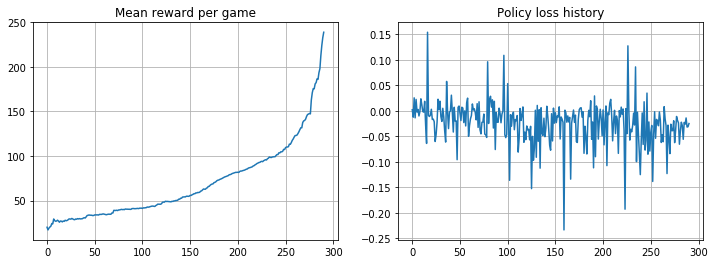
plt.subplot(1, 2, 1)
plt.title("Mean reward per game")
plt.plot(mean_rw_history)
plt.grid()
plt.subplot(1, 2, 2)
plt.title("Policy loss history")
plt.plot(np.array(losses))
plt.grid()
plt.show()
break #next episode
### next step
state = new_state
四、使用训练好的网络进行实验
点击查看代码
total_rewards = 0
for episode in range(100):
    state = env.reset()
    episode_reward = 0
    while True:
        action_prob_t = agent.get_action_probs(state[None,:])
        action = agent.sample_action(action_prob_t)
        new_state, reward, done, info = env.step(action)
        episode_reward += reward
        if done:
            total_rewards += episode_reward
            break
        state = new_state
print("Score over 100 consecutive trials: ", total_rewards/100.)