
在文章循环神经网络RNN介绍中提到了一种非同步输出的many to many的结构,它输入的是一个序列,输出的也是一个序列,但两个序列的长度不一定相等,这种结构也叫做Seq2Seq模型。如下图所示,通常使用编码器-解码器 (Encoder-Decoder) 架构对其进行搭建:
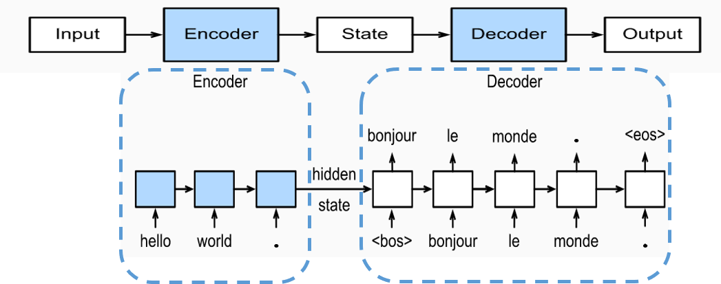
编码器对输入进行编码,并将得到的最终状态输入到解码器中,由解码器进行解码获得对应的输出。在Seq2Seq模型中编码器和解码器通常选择RNN网络或者它的变体 (例如LSTM、GRU)。但是这种Seq2Seq模型还存在一个问题,以上图中的例子为例,它将“Hello world.”翻译为“Bonjour le monde.”,实际上是“Bonjour”对应“Hello”,“monde” 对应“world”,但是Seq2Seq模型只是将输入的句子转化为一个最终状态输入到解码器中,很难直接学习到这种对应关系。为解决这一问题,需引入注意力机制 (Attention Mechanism) 加入到Seq2Seq模型中。
注意力机制
注意力机制的目的是在生成输出序列的每一步时考虑整个输入序列,选出对该输出步影响最大的关键输入部分,而忽略其它不重要的输入部分。注意力机制的结构如左图所示,将注意力层的输入记为一个query(用\boldsymbol{q}表示),将输出output记为\boldsymbol{o},将嵌入注意力层的网络的记忆表示为n个键-值(key-value)对,记为\boldsymbol{(k_1, v_1), (k_2, v_2), \cdots, (k_n, v_n)}。
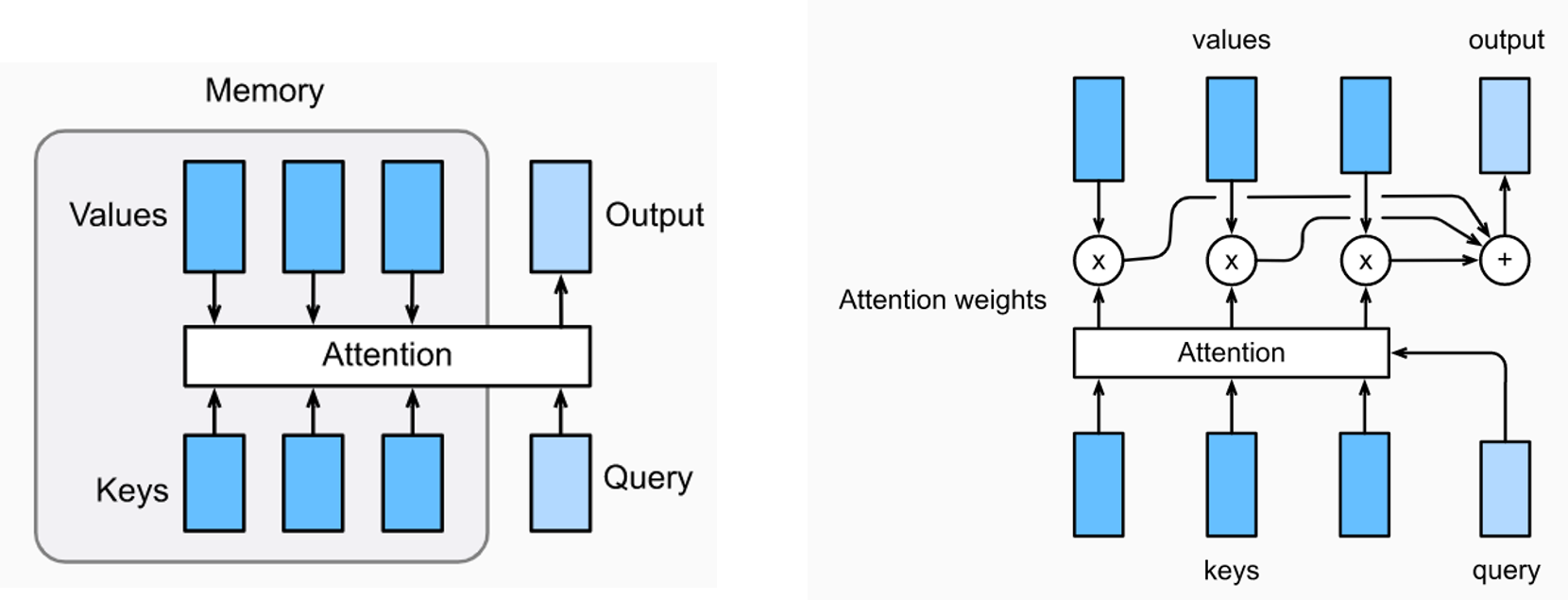
注意力层的具体计算方法如右图所示,对每个输入\boldsymbol{q},结合网络记忆\boldsymbol{k_i}计算出权重系数\alpha_i:\large r_i = F(\boldsymbol{q}, \boldsymbol{k_i}),\space\space \alpha_i=\frac{\large e^{r_i}}{\large \sum_{j=1}^n e^{r_j}},\space\space i=1,2,\cdots,n其中函数F通常为一个浅层的神经网络。计算出权重系数后注意力层的输出可以写为\large \boldsymbol{o}=\sum_{i=1}^{n}\alpha_i \boldsymbol{v_i}
接下来通过一个实例介绍在Seq2Seq模型中如何引入注意力机制,该实例的目的是将不同类型的英文日期表述转化为固定的格式"YYYY-MM-DD",例如:

使用的数据集可以点击此链接下载,提取码为4y8l。首先进行数据读取和处理:
点击查看代码
import numpy as np
from keras.utils import to_categorical

with open('date.txt','r') as f:
    dataset = eval(f.read())
### character dict for human date format
human_vocab = {' ': 0, '.': 1, '/': 2, '0': 3, '1': 4, '2': 5, '3': 6, '4': 7, '5': 8, '6': 9, '7': 10, '8': 11, '9': 12,
               '<pad>': 36, '<unk>': 35, 'a': 13, 'b': 14, 'c': 15, 'd': 16, 'e': 17, 'f': 18, 'g': 19, 'h': 20, 'i': 21,
               'j': 22, 'l': 23, 'm': 24, 'n': 25, 'o': 26, 'p': 27, 'r': 28, 's': 29, 't': 30, 'u': 31, 'v': 32, 'w': 33, 'y': 34}
### character dict for machine date format YYYY-MM-DD
machine_vocab = {'-': 0, '0': 1, '1': 2, '2': 3, '3': 4, '4': 5, '5': 6, '6': 7, '7': 8, '8': 9, '9': 10}
inv_machine_vocab = {0: '-', 1: '0', 2: '1', 3: '2', 4: '3', 5: '4', 6: '5', 7: '6', 8: '7', 9: '8', 10: '9'}
### process data
def string_to_int(string, length, vocab, is_human):
    string = string.lower()
    string = string.replace(',','')
    if len(string) > length:
        string = string[:length] #truncate string if string is too long
    # transform string to a list of integers. if character not in the vocab, replace it with <unk>
    rep = list(map(lambda x: vocab.get(x, vocab['<unk>']), string)) if is_human else list(map(lambda x: vocab.get(x), string))
    # pad short string with <pad>
    if len(string) < length:
        rep += [vocab['<pad>']] * (length - len(string))
    return rep

def preprocess_data(dataset, human_vocab, machine_vocab, Tx, Ty):
    m = len(dataset)
    X, Y = zip(*dataset) #(m,), (m,)
    X = np.array([string_to_int(i, Tx, human_vocab, is_human=True) for i in X]) #(m, Tx)
    Y = np.array([string_to_int(t, Ty, machine_vocab, is_human=False) for t in Y]) #(m, Ty)
    Xoh = np.array(list(map(lambda x: to_categorical(x, num_classes=len(human_vocab)), X))) #(m, Tx, len(human_vocab))
    Yoh = np.array(list(map(lambda x: to_categorical(x, num_classes=len(machine_vocab)), Y))) #(m, Ty, len(machine_vocab))
    return X, Y, Xoh, Yoh

Tx, Ty = 30, 10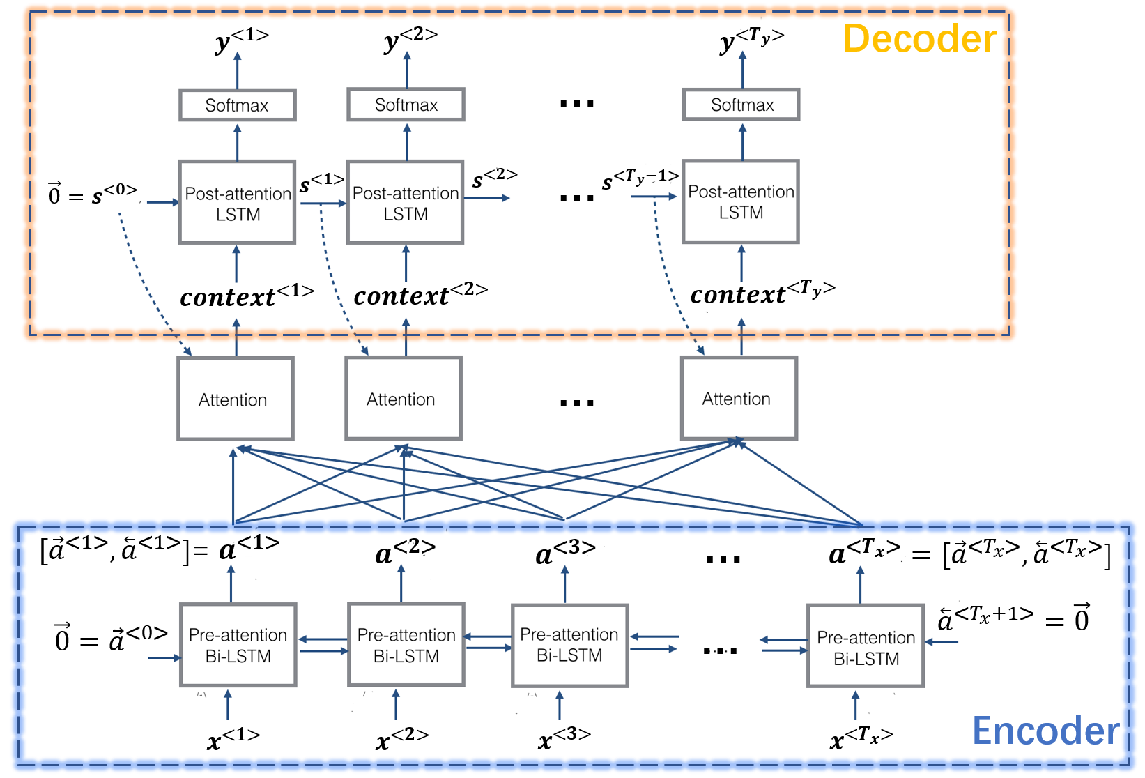
X, Y, Xoh, Yoh = preprocess_data(dataset, human_vocab, machine_vocab, Tx, Ty)该问题的模型架构如下图所示,它的编码器部分由双向(Bidirectional) LSTM网络组成,每步输出为\boldsymbol{a^{<i>}}=\left[\boldsymbol{\overrightarrow{a}^{<i>}}, \boldsymbol{\overleftarrow{a}^{<i>}}\right],其中\boldsymbol{\overrightarrow{a}^{<i>}}为正向LSTM的输出,\boldsymbol{\overleftarrow{a}^{<i>}}为反向LSTM的输出;解码器部分由LSTM网络组成,每步的输出为\boldsymbol{s^{<i>}},并通过全连接层转化为最终的输出\boldsymbol{y^{<i>}}。此外,该架构中还引入了注意力机制,注意力层的输出为\boldsymbol{context^{<i>}}。一般来说,解码器每步也会有自己的输入\boldsymbol{d^{<i>}},引入注意力机制后解码器的输入变为\left[\boldsymbol{d^{<i>}}, \boldsymbol{context^{<i>}}\right],这里为了简化模型在该问题中没有考虑\boldsymbol{d^{<i>}}。
模型整体架构的代码为:
点击查看代码
from keras.layers import Bidirectional, Input, LSTM, Dense
from keras.models import Model

### Defined shared layers as global variables
n_a = 32 # number of units for the pre-attention, bi-directional LSTM's hidden state 'a'
n_s = 64 # number of units for the post-attention LSTM's hidden state "s"
post_attention_LSTM_cell = LSTM(n_s, return_state = True) # post-attention LSTM
output_layer = Dense(len(machine_vocab), activation="softmax")

### Model architecture
def model(Tx, Ty, n_a, n_s, human_vocab_size, machine_vocab_size):
    X = Input(shape=(Tx, human_vocab_size))
    s0 = Input(shape=(n_s,), name='s0') #define s0 (initial hidden state)
    c0 = Input(shape=(n_s,), name='c0') #define c0 (initial cell state)
    s = s0
    c = c0
    outputs = [] # Initialize empty list of outputs, final shape: Ty np arrays with shape (m, len(machine_vocab))
    # Step 1: Define pre-attention Bi-LSTM.
    a = Bidirectional(LSTM(units=n_a, return_sequences=True))(X) #(m, Tx, 2*n_a)
    # Step 2: Iterate for Ty steps
    for t in range(Ty):
        # Step 2.A: Perform one step of the attention mechanism to get the context vector at step t
        context = one_step_attention(a, s) #the attention layer is defined below, (m, 1, 2*n_a)
        # Step 2.B: Apply the post-attention LSTM cell to the context vector
        s, _, c = post_attention_LSTM_cell(context, initial_state=[s,c]) #(m, n_s), (m, n_s)
        # Step 2.C: Apply Dense layer to the hidden state output of the post-attention LSTM
        out = output_layer(s) #(m, len(machine_vocab))
        # Step 2.D: Append "out" to the "outputs" list
        outputs.append(out)
    # Step 3: Create model instance
    model = Model(inputs=[X,s0,c0], outputs=outputs)
    return model
针对注意力层的计算过程如下图所示:
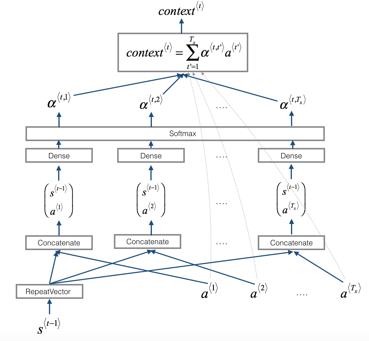
类比文章上一部分提到的注意力层的计算方法,此时网络记忆可写为\boldsymbol{k_{t^\prime}}=\boldsymbol{v_{t^\prime}}=\boldsymbol{a^{<t^\prime>}},\space\space t^\prime =1,2,\cdots,T_x注意力层每步的输入为解码器中LSTM的前一步的输出,即\boldsymbol{q_t}=\boldsymbol{s^{<t-1>}}, \space\space t=1,2,\cdots,T_y注意力层每步的输出\boldsymbol{o_t}=\boldsymbol{context^{<t>}},计算公式为\begin{cases}r^{<t,t^\prime>}=F(\boldsymbol{q_t}, \boldsymbol{k_{t^\prime}})=F(\boldsymbol{s^{<t-1>}}, \boldsymbol{a^{<t^\prime>}}), \space\space t^\prime = 1,2,\cdots,T_x \\ \alpha^{<t,t^\prime>}=\frac{\large e^{r^{<t,t^\prime>}}}{\large \sum_{j=1}^{T_x} e^{r^{<t,j>}}},\space\space t^\prime =1,2,\cdots,T_x \\ \boldsymbol{context^{<t>}} = \sum_{t^\prime =1}^{T_x}\alpha^{<t,t^\prime>}\boldsymbol{v_{t^\prime}} = \sum_{t^\prime =1}^{T_x}\alpha^{<t,t^\prime>}\boldsymbol{a^{<t^\prime>}}\end{cases}其中F为一个浅层的全连接神经网络。注意力层的代码为:
点击查看代码
from keras.layers import Concatenate, Dot, RepeatVector, Activation
import keras.backend as K

### Define a custom softmax function for convenient use in attention layer
def softmax(x, axis=1):
    """
    Arguments:
    x -- Tensor.
    axis -- Integer, axis along which the softmax normalization is applied.
    """
    ndim = K.ndim(x)
    if ndim == 2:
        return K.softmax(x)
    elif ndim > 2:
        e = K.exp(x - K.max(x, axis=axis, keepdims=True))
        s = K.sum(e, axis=axis, keepdims=True)
        return e / s
    else:
        raise ValueError('Cannot apply softmax to a tensor that is 1D')

### Defined shared layers as global variables
repeator = RepeatVector(Tx)
concatenator = Concatenate(axis=-1)
# [densor1,densor2] is F
densor1 = Dense(10, activation = "tanh")
densor2 = Dense(1, activation = "relu")
activator = Activation(softmax, name='attention_weights') #using a custom softmax(axis = 1)
dotor = Dot(axes = 1)

### Perform one step of attention
def one_step_attention(a, s_prev):
    """
    Arguments:
    a -- hidden state output of the Bi-LSTM, numpy-array of shape (m, Tx, 2*n_a)
    s_prev -- previous hidden state of the (post-attention) LSTM, numpy-array of shape (m, n_s)
    """
    s_prev = repeator(s_prev) #(m, Tx, n_s)
    concat = concatenator([a, s_prev]) #(m, Tx, 2*n_a+n_s)
    e = densor1(concat) #(m, Tx, 10)
    energies = densor2(e) #(m, Tx, 1)
    alphas = activator(energies) # compute the attention weights, (m, Tx, 1)
    context = dotor([alphas, a]) #(m, 1, 2*n_a)
    return context
模型训练和预测的代码为:
|
1 2 3 4 5 6 7 8 9 10 11 12 13 14 15 16 17 18 19 20 21 22 23 |
from keras.optimizers import Adam ### Train model = model(Tx, Ty, n_a, n_s, len(human_vocab), len(machine_vocab)) model.summary() opt = Adam(lr=0.005, beta_1=0.9, beta_2=0.999, decay=0.01) model.compile(optimizer=opt, loss='categorical_crossentropy', metrics=['accuracy']) s0 = np.zeros((m, n_s)) c0 = np.zeros((m, n_s)) outputs = list(Yoh.swapaxes(0,1)) #(m, Ty, len(machine_vocab)) --> Ty np arrays with shape (m, len(machine_vocab)) model.fit([Xoh, s0, c0], outputs, epochs=30, batch_size=100) ### Test EXAMPLES = ['3 May 1979', '3rd of August 2016', 'Tue 16 Jul 2007', 'Saturday May 9 2018', 'March 3 2001', 'Jun 9th 2001', '09/19/1996'] for example in EXAMPLES: source = string_to_int(example, Tx, human_vocab, is_human=True) source = np.array(list(map(lambda x: to_categorical(x, num_classes=len(human_vocab)), source)))[None,:,:] #(1, Tx, len(human_vocab)) prediction = model.predict([source, s0, c0]) #a list of Ty np arrays with shape (1, len(machine_vocab)) prediction = np.argmax(prediction, axis = -1) #(Ty, 1) output = [inv_machine_vocab[int(i)] for i in prediction] print("source:", example) print("output:", ''.join(output),"\n") |